Airport

Introduction

Air passenger travel to/from the Raleigh-Durham International Airport (RDU) is captured by the air passenger model.

A limited amount of data on air passengers is available. The modeling approach is therefore straightforward and requires a handful of assumptions. The available data is passive movements recorded from StreetLight Data. The benefits of this data is they provide a reasonable signal of movements to/from the airport. The drawbacks of this data are as follows: It does not distinguish between airport employees and air passengers. It cannot distinguish between trip legs, for example the movement from home to an off-airport parking location and the movement from the off-airport parking location to the airport terminal. And it cannot distinguish between residents of the Triangle region and visitors to the Triangle region.

StreetLight Data Summaries

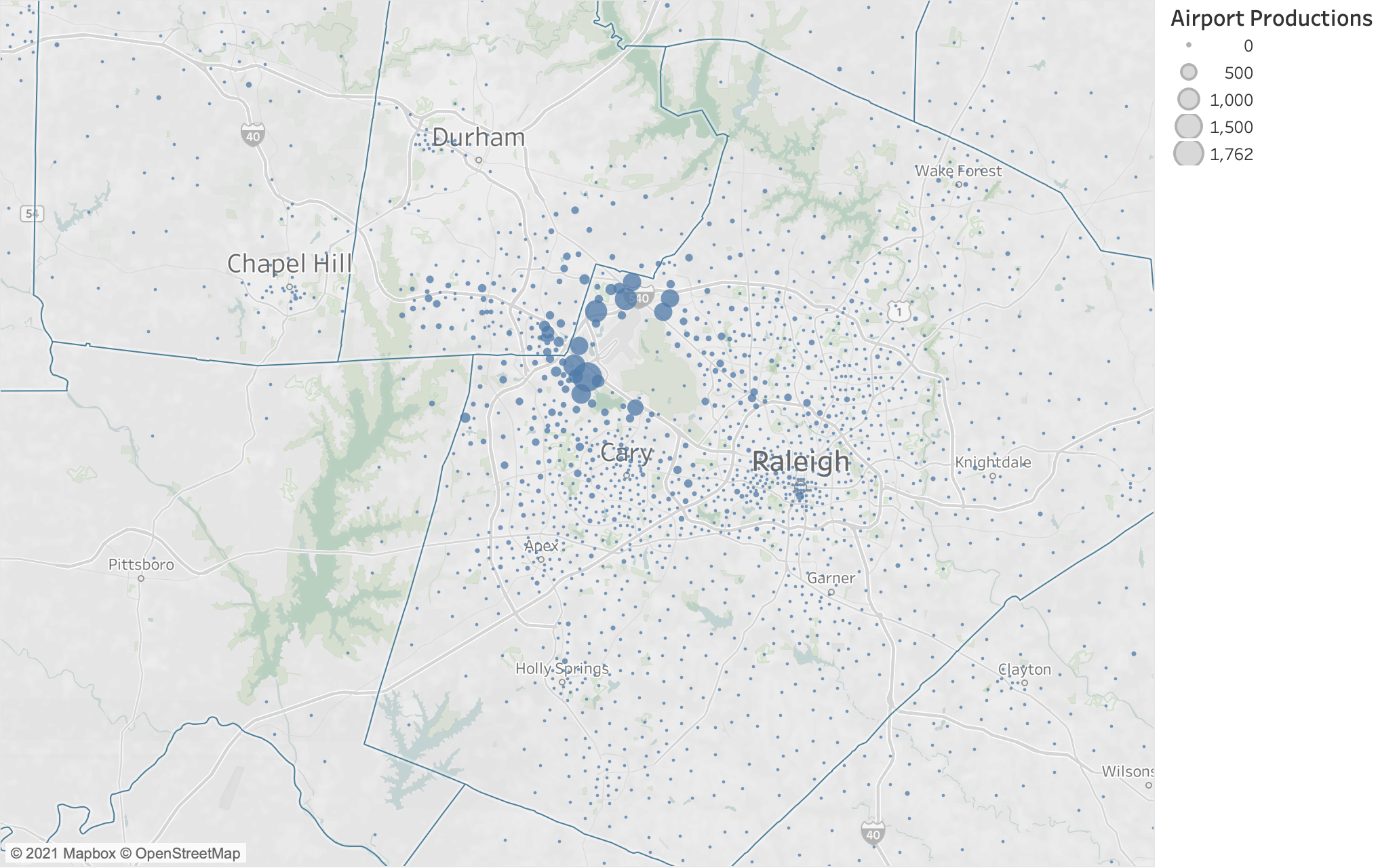
The map below shows the distribution of trip productions to RDU per the StreetLight data. As expected, the data shows large amounts of activity in the zones surrounding the airport. For an air passenger model, we are less interested in the movement from, say, the off-airport parking facility to the airport, than we are the movement from a home or workplace to the off-airport parking facility. Ideally, an airport model would explicitly represent each movement. For the simple model being developed here, we want to focus on the primary (and longer) movement.

StreetLight “Raw” Productions

To ameliorate the impact of near-airport movements on the estimation of production models intended to locate the “true” origin of air passenger movements, we censor the “raw” StreetLight productions to a maximum value of 200. The map of truncated productions is shown in the map below. (Because the “raw” values are scaled to match the RDU enplanements, the map below shows some locations with a value larger than 200).

StreetLight Censored Productions

Production Modeling

The goal of the air passenger production model is to generate travel from home and employment locations to the airport. Because all trips are destined to RDU, the production model acts as both a trip generation and trip distribution model.

To begin the data exploration and model estimation stage, we summarize the correlations between the socio-economic data expected to be relevant and airport productions. These correlations are shown in the table below.

Correlations

term	airport_productions
employment	0.250
high_paying_jobs	0.228
Retail	0.206
Pct_Worker	0.202
Service_RateHigh	0.191
Industry	0.173
Office	0.163
workers	0.122
HH	0.118
Service_RateLow	0.099
PctHighEarn	0.086
Total_POP	0.079
high_paying_jobs_distance	0.069
Median_Inc	0.030
hotel_rooms	-0.002
BuildingS_NCSU	-0.009
Other_NonInst_GQ	-0.010
Inst_GQ	-0.011
Stud_GQ	-0.018
dist_to_airport_miles	-0.231
airport_productions	NA

The above table shows correlations between airport productions and the variables we would expect and like to be correlated with airport productions, including workers, employment, and high income employment.

Using the correlations as a guide, we estimate a series of linear regression models in a search for a parsimonious balance between model fit and logical coefficients.

Model Estimation Results

Numerous model estimations were conducted to find the preferred specification shown below. The preferred specification includes high paying jobs, which is the number of high paying jobs in each TAZ. A second term that interacts high paying jobs with distance to the airport is included as well, which reduces the number of productions for high earners at greater distances from the airport.

The preferred specification includes employment which captures movements to/from work locations to the airport. The preferred specification collapses the employment categories. Specifications with employment separated by industry did not always reveal logical coefficients (e.g., a larger coefficient on industrial employment than office employment).

Other, non-preferred specifications are included in the tabs below.

Preferred

variable	estimate	statistic	p.value
employment	0.0143	9.3718	0
high_paying_jobs	0.0470	13.4705	0
high_paying_jobs_distance	-0.0036	-16.0087	0
workers	0.0283	22.1940	0
Adjusted R-squared	0.4332	NA	NA

Model 01

variable	estimate	statistic	p.value
intercept	1.1001	1.0929	0.2746
employment	0.0148	16.6428	0.0000
workers	0.0247	13.2494	0.0000
Adjusted R-squared	0.1789	NA	NA

Model 02

variable	estimate	statistic	p.value
intercept	1.3877	1.5461	0.1222
high_paying_jobs	0.0789	17.7869	0.0000
high_paying_jobs_distance	-0.0045	-20.0489	0.0000
hotel_rooms	0.0179	0.2506	0.8022
Industry	0.0328	6.8770	0.0000
Office	-0.0135	-4.5808	0.0000
Retail	0.0322	10.8586	0.0000
Service_RateHigh	0.0774	8.3349	0.0000
workers	0.0243	14.7856	0.0000
Adjusted R-squared	0.3659	NA	NA

Model 03

variable	estimate	statistic	p.value
intercept	2.6323	2.7835	0.0054
employment	0.0132	8.3809	0.0000
high_paying_jobs	0.0479	13.6943	0.0000
high_paying_jobs_distance	-0.0036	-16.2064	0.0000
hotel_rooms	-0.0023	-0.0310	0.9753
workers	0.0250	14.3636	0.0000
Adjusted R-squared	0.2833	NA	NA

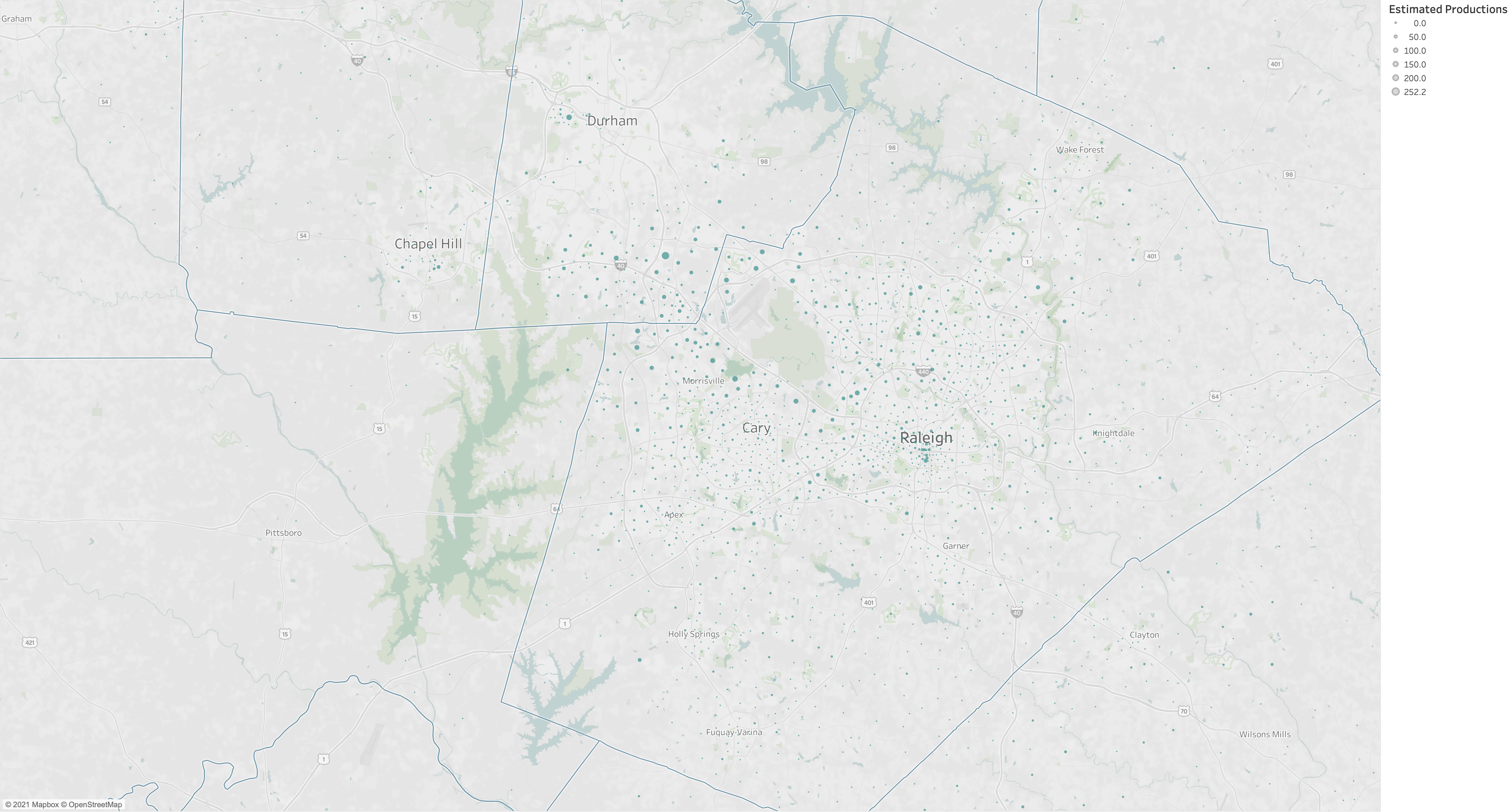
Predicted Productions

The map below plots the predicted airport productions. In model application, the calculated productions will be scaled to airport attractions, which is the number of enplanements at RDU entered by the model user. The current chart assumes 15343 daily enplanements. It is also possible for the regression model to return a negative number of enplanements due to the negative coefficient on the high paying jobs and distance interaction term. These productions have been censored at zero and will need to be similarly censored in model application.

The chart below plots the adjusted observed productions (truncated at 200 times the scaling necessary to matche the target attractions) against the estimated productions.

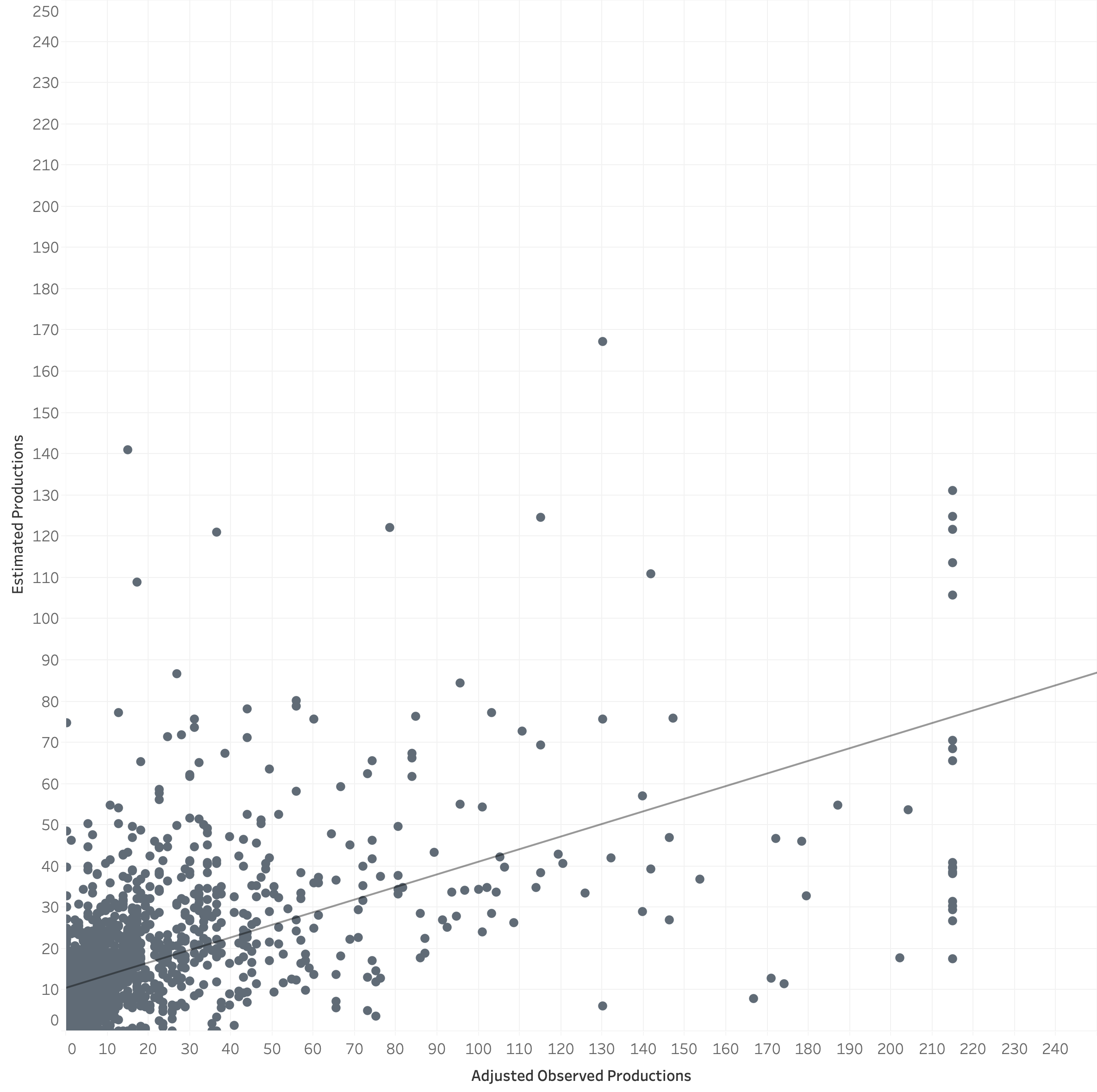
The chart below shows the adjusted observed and estimated trip length frequency distributions for movements to the airport. The model estimates longer trips than the StreetLight data. This is expected because the StreetLight data will, in many cases, fail to capture the true origin of the movement, misunderstanding stops at gas stations, cell phone lots, rental car facilities, etc, as the origin.

Diurnal Factors

The table below summarizes the production to airport and airport to production trips by time of day, based on the StreetLight data.

P to A Diurnal Factors from StreetLight

purpose	day_part	share
To Airport	1: Early AM (12am-6am)	0.170
To Airport	2: Peak AM (6am-10am)	0.226
To Airport	3: Mid-Day (10am-3pm)	0.293
To Airport	4: Peak PM (3pm-7pm)	0.225
To Airport	5: Late PM (7pm-12am)	0.085
To Airport	All	1.000

A to P Diurnal Factors from StreetLight

purpose	day_part	share
From Airport	1: Early AM (12am-6am)	0.064
From Airport	2: Peak AM (6am-10am)	0.132
From Airport	3: Mid-Day (10am-3pm)	0.302
From Airport	4: Peak PM (3pm-7pm)	0.283
From Airport	5: Late PM (7pm-12am)	0.219
From Airport	All	1.000

The time periods used for the StreetLight extraction do not directly align with the time periods used for the updated travel model. By assuming a uniform distribution across the StreetLight time periods, we can create the below diurnal factors using the StreetLight data and model time periods.

P to A Travel Model Diurnal Factors

purpose	direction	period	share
To Airport	P to A	AM	0.113
To Airport	P to A	MD	0.377
To Airport	P to A	PM	0.155
To Airport	P to A	NT	0.354
To Airport	P to A	All	1.000

A to P Travel Model Diurnal Factors

purpose	direction	period	share
From Airport	A to P	AM	0.066
From Airport	A to P	MD	0.370
From Airport	A to P	PM	0.195
From Airport	A to P	NT	0.369
From Airport	A to P	All	1.000

Mode Choice

The StreetLight Data does not provide insight to the mode choice decision made by air passengers. As such, no information is available to base a mode choice model on. We therefore will add the airport trips to the home-based other trip purpose prior to mode choice and use the home-based other model to simulate the mode choice decision for air passengers.