Household Survey Processing
Introduction
The Institute for Transportation Research and Education (ITRE) on behalf of the Triangle Region stakeholders, began conducting rolling household travel surveys in 2016. For the TRMG2 estimation, both the 2016 and 2018 surveys were available. This page documents the combination of those surveys along with any general processing steps not specific to a particular model.
This survey includes tables describing households, persons, trips, and vehicles. They are linked together with IDs so that the entire travel diary for each person can be created. Survey processing checks for potential problems in the survey and corrects those it finds. It also creates numerous calculated fields that are specific to travel demand modeling. For example, we flip origins and destinations into productions and attractions. This is not something we want to ask each person in the survey, but is needed to properly estimate resident trip production models. Additionally, trips are organized into tours, activity types are condensed, and other steps are taken to support subsequent model estimation.
Survey combination
When RSG delivered the 2018 survey, they provided weighting and expansion factors for 2018 using two data sets:
- Only the 2018 samples
- A combination of 2016 and 2018 samples
The combined data set expansion was controlled using 2018 American Community Survey (ACS) marginals. For TRMG2, with a 2016 base year, these weights were deemed close enough. For example, the table below shows that the original and combined weights for the 2016 records produce effectively the same distribution of household size.
| HH Size | 2016 weights | Combined Weights |
|---|---|---|
| 1 | 27.1% | 26.2% |
| 2 | 33.7% | 33.7% |
| 3 | 16.6% | 17.4% |
| 4 | 14.2% | 14.7% |
| 5 | 8.3% | 7.9% |
For models where absolute counts of households matter (like trip production), the weights will be scaled down to match the 2016 socio-economic (SE) data’s total household count. For models focused on percentages (e.g. destination and mode choice), the raw weights will be used in estimation and calibration. This includes target creation for mode choice.
Household table
The 2016 survey household table did have slight differences in the field names and definitions from the 2018 survey. Compared to the person and trip tables, the household table was easy to combine and did not result in losing any information.
Person table
The person table changed substantially between 2016 and 2018. As an example, race included 6 categories in 2016 and was contained in a single column. In 2018, race only had 5 categories and was contained in 5 separate binary columns (e.g. race_white = 1 or 0). These formats had to be rectified, and the “Two+” race category from 2016 collapsed into “Other”, before the tables could be combined.
In addition, some fields in the 2016 table were not present in 2018 (and vice versa). The num_transitpass field kept track of how many transit passes the person used per week in 2016. This field was dropped in 2018. While several fields were dropped, none were critical to model estimation.
Trip table
Similar to the person table, the trip tables from 2016 and 2018 contained different fields and field definitions, which complicated the combination process. Importantly, the definition of activity purpose changed slightly between the two years. Both columns were left in the combined table, to be processed in the next step.
Basic checks
A common task in household survey processing is to remove households for various reasons. For instance, travel models estimate weekday travel, so households surveyed on the weekend must be removed. Households may have incomplete travel diaries, be located outside the model region, or have other issues that requires removal from the estimation data set. This section documents that process and the removal of specific data records.
Day of week
Due to careful survey design, none of the Triangle households were surveyed on the weekend. The chart below shows the days surveyed (1 is Monday).

Starting in 2018, the survey process was modified to only collect travel diaries in the middle of the week, excluding travel on Monday and Friday. These days often display differences in trip rates as compared to the other days of the week, perhaps due to .holidays, vacations, alternative work schedules, or other reasons. The hypothesis of differences in trip rates on Monday and Friday as compared to mid-week travel (Tuesday through Thursday) was evaluated by applying a t-test to the average trip rate per household for each day of week category. The result suggests that trip making shows no significant difference between the day of week categories, leading to the decision to retain all surveyed households in the estimation data set.
| Parameter | Value |
|---|---|
| Average Trips/HH (Mon/Fri) | 9.14 |
| Average Trips/HH (Midweek) | 8.82 |
| t-stat | 1.59 |
| p.value | 0.11 |
Household locations
It is also important to make sure that only households in the model region are used for estimation. This ensures that the model reflects the travel patterns that make the Triangle unique. The map below shows the locations of all households included in the survey. Each falls within the model boundary, and no households had to be dropped.
Incomplete records
Travel surveys such as the National Household Travel Survey include households where only half of the household members filled out a travel diary. These households cannot be used in estimation for certain sub models (e.g. trip production), because the household reports fewer trips than what actually took place. Looking at the survey data cannot determine if people failed to fill out a travel diary; they may have simply taken no trips on the survey day. Instead, the survey documentation from RSG reports that only fully-reported households were included in the data set.
Survey weights
It is important to check the weighting and expansion of a survey for extreme weight values. A large weight indicates that they survey failed to collect adequate samples from a specific segment of the population, which can bias model estimation and lead to poor predictive power. To check the weights, they must first be normalized based on the expected average weight per sample. A simple comparison of two hypothetical surveys explains why:
- A survey with 100 samples of a population of 100,000: Average weight = 1,000
- A survey with 1000 samples of a population of 100,000: Average weight = 100
A household weight of 1,000 in the first survey is reasonable based on the number of samples, but it is 10 times the expected weight in the second survey. For the 2016+2018 combined survey, the average weight is shown below.
| Year | Samples | Total Households | Average Weight |
|---|---|---|---|
| 2016 | 4,169 | 526,463 | 126 |
| 2018 | 1,498 | 166,515 | 111 |
| Total | 5,667 | 692,978 | 122 |
The first histogram below shows the distribution of weights divided by the mean weight. While the largest weight is 15x the mean weight, this is an outlier and most are within 6x. This is a reasonable result and indicates a well-designed sample plan that collected a representative number of households in all the demographic groups of interest.
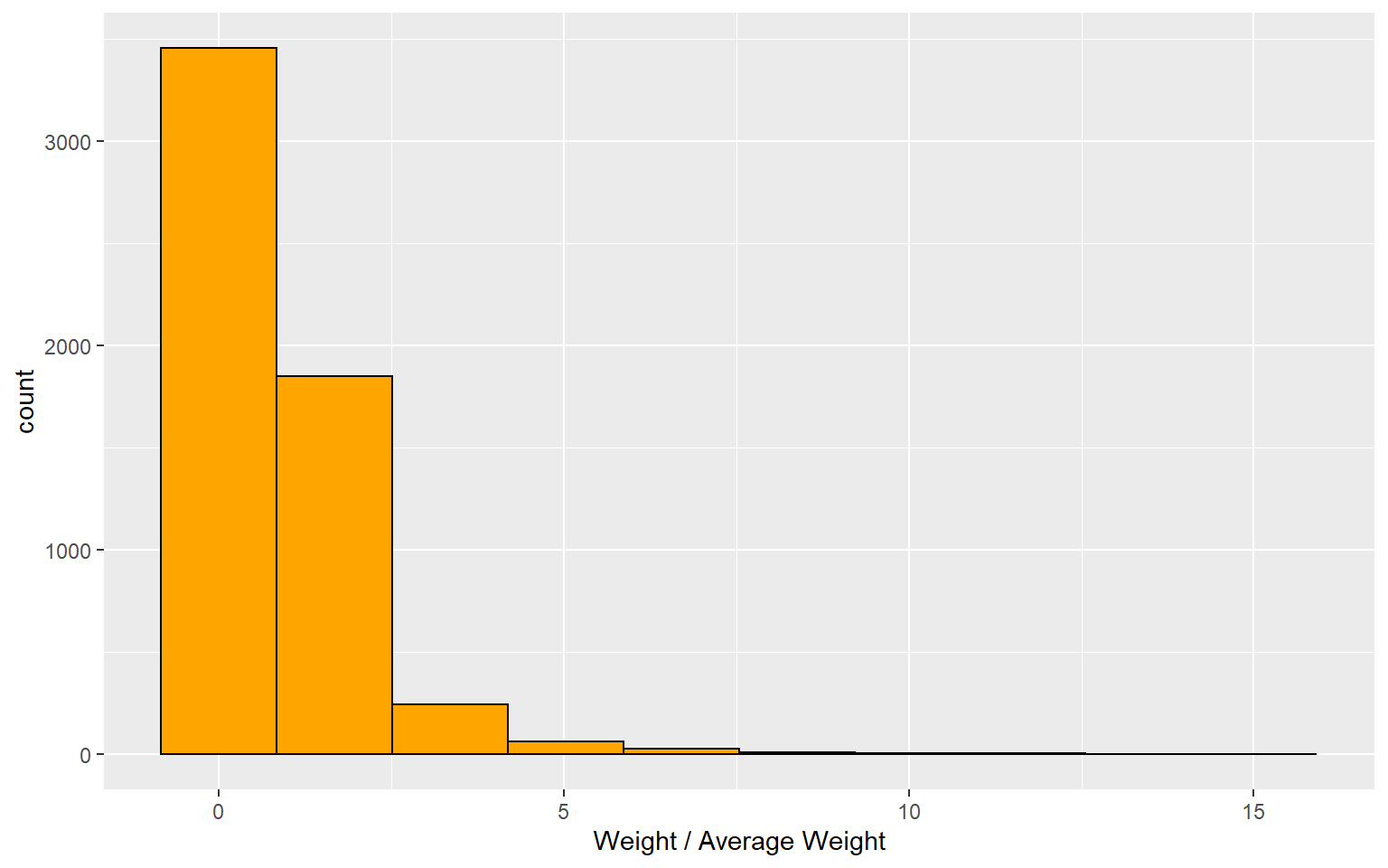
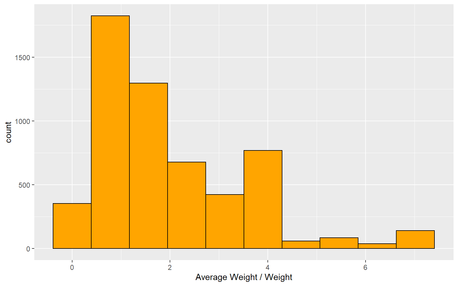
The histogram above is good for identifying weights that are too large, but does not help identify those that are very small. Small weights are not problematic like large weights, but they imply oversampling of a target demographic, which could inform future collection efforts. The second histogram below inverts the factor above and divides the average weight by the individual household weights. Large numbers in this histogram would indicate the presence of small weights. The smallest weight (17.3) is 14% of the average weight (1 / .14 = 7.14 in the histogram below). This suggests a modest over sample, but well within reason.
After a review of the RSG expansion procedure combined with the review of weights described above, Caliper determined that the weights were appropriate for use in model estimation.
Income imputation
The survey provides income at two levels of aggregation: 10 categories or 5. RSG imputed incomes for the broad category in order to use ACS income information during survey expansion. The imputation:
- Further stratified category 5 ($100k+) into those above and below $150k.
- Imputed incomes for those households that did not report.
In order to preserve all the records in the survey, the Caliper team used the imputed, broad categories of income. The table below shows the count of samples by the original and imputed categories.
| Original | Count |
|---|---|
| Under $25,000 | 572 |
| $25,000-$49,999 | 914 |
| $50,000-$74,999 | 939 |
| $75,000-$99,999 | 783 |
| $100,000 or more | 1839 |
| Prefer not to answer | 620 |
| Imputed | Count |
|---|---|
| Under $25,000 | 628 |
| $25,000-$49,999 | 1029 |
| $50,000-$74,999 | 1091 |
| $75,000-$99,999 | 895 |
| $100,000-$149,999 | 1170 |
| $150,000 or more | 854 |
A full discussion of their income imputation can be found in the survey documentation. They used ordinal logistic regression to predict income categories based on household features like size and number of workers (among others).
Trip processing
Trip processing for the TRMG2 departs from the common approach of categorizing trips by trip purpose. Instead, trips are categorized by
- Tour Type: Whether the trip takes place on a work or non-work tour.
- Homebased: Whether one end of the trip is home or not.
- Activity: What the person does after making the trip (similar to traditional trip purpose)
- Duration: How long the person spends at their destination.
These new classifications provide more insight into travel behavior compared to traditional trip purposes.
Segmenting trips by tour type is helpful and justified for multiple reasons. Both non-home-based (NHB) and home-based other (HBO) trips on work tours have distinct mode shares, temporal and spatial distributions from NHB and HBO trips on non-work tours. Trips on work tours generally tend to have mode shares more akin to home-base work (HBW) trips with more drive alone and transit trips. HBO trips on work tours are concentrated in the AM and PM peaks like HBW, while HBO trips on nonwork tours gradually increase through the day to a peak during the mid-day period and slowly taper off. NHB trips on work tours also have a distinct triple peak pattern with concentrations around the lunch hour as well as the AM and PM peaks; whereas, NHB trips on nonwork tours are distributed through the day similarly to HBO trips on nonwork tours with a unimodal distribution. Spatially, trips on work tours are more tied to general employment (and enrollment in the AM) compared to trips on nonwork tours which are more concentrated around retail. Traditional trip purposes capture some of the differences between trips on work tours and nonwork tours by segmenting HBW and NHBW separately from HBO and NHBO, but actually segmenting by tour type can better preserve these differences. For example, if a person drops off a child at school and then gets gas on their way to work, the traditional treatment would classify the trip from school to the gas station as NHBO and lose the understanding that it was actually part of a work tour and therefore more likely to be drive alone in the AM period.
Segmentation by home-based and non-home-based is a fundamental and necessary aspect of trip-based travel demand modeling. It is similar to the segmentation between tour level (tour mode, tour destination) and trip level (trip mode, intermediate stop location) choices in activity-based models.
Segmentation by activity type is also traditional and standard in both trip- based and activity-based models since mode, temporal and spatial distributions do vary by activity type.
Segmentation by duration is less common, but a growing practice (in part because it is more easily supported by big data than segmentation by activity type). In some cases activity duration can provide meaningful information and distinct distributions by mode, time-of-day, and location even after accounting for tour and activity type. This was the case for discretionary trips on nonwork tours in the Triangle. Long activity discrectionary trips were twice as long as their short counterparts, which were five times as likely to be by walk.
The following sections provide more detail on the segmentation for the TRM.
Activity types
As described above, the activity type describes what the activities a person is performing throughout the day. The survey provides many categories for activity type, but the Caliper collapsed them into the types shown below.
- H: Home (non-work activities at home)
- W: Work
- WR: Work-related (e.g. making a delivery)
- PreK: Attend school (Pre-Kindergarten)
- K12: Attend school (Kindergarten through 12th grade)
- U: Attend school (University or College)
- SHP: Shop
- EAT: Dining out
- PU: Pick up
- DO: Drop off
- X: Transfer modes (e.g. at a bus stop)
- OM: Other maintenance
- OMED: Other medical
- OD: Other discretionary
The table below shows how the activity types (for both years) were collapsed into the types above.
| Activity Code | 2016 Description | 2016 Equivalence |
|---|---|---|
| 1 | At home activity, not working (for pay) or schooling | H |
| 2 | Working (for pay) at work or home | W |
| 3 | Work-related: delivering goods or services | WR |
| 4 | Other work-related activity (meeting, visit, sale call, etc.) | WR |
| 5 | Attend school/class | SCH |
| 6 | Other school-related activity | OD |
| 7 | Routine shopping (grocery, get gas, clothing, convenience store, household maintenance, etc.) | SHP |
| 8 | Shopping for major purchase/specialty item (appliance, electronics, new vehicle, major household repairs, etc.) | SHP |
| 9 | Dining out/take-out/coffee (eat at restaurant, get take-out/fast-food) | EAT |
| 10 | Pick someone up | PU |
| 11 | Drop someone off | DO |
| 12 | Change type of transportation/Transfer to (take bus, airplane, park car or pick up parked car if walk 2+ blocks, etc.) | X |
| 13 | Household errands (bank/ATM, post office, dry cleaning, car services, etc.) | OM |
| 14 | Personal business (visit government office, attorney, accountant, etc.) | OM |
| 15 | Medical visit (doctor, dentist, etc.) | OMED |
| 16 | Recreation/entertainment (walk the dog, exercise/workout, go to a movie) | OD |
| 17 | Social (visit friends/relatives) | OD |
| 18 | Religious, civic, or volunteer | OD |
| 19 | Other (not at home) | OD |
| Activity Code | 2018 Description | 2018 Equivalence |
|---|---|---|
| 1 | At home activity (including school), EXCLUDE working for pay | H |
| 2 | At home, working for pay | W |
| 3 | At work (not home), working for pay | W |
| 4 | Other work-related activity (e.g., meeting, site visit, sales call, etc.) | WR |
| 5 | Attend school/class | SCH |
| 6 | Other school-related activity | OD |
| 7 | Routine shopping (e.g., grocery, get gas, clothing, convenience store, household maintenance, etc.) | SHP |
| 8 | Shopping for major purchase/specialty item (e.g., appliances, electronics, new vehicle, major household repairs, etc.) | SHP |
| 9 | Dining out/take-out/coffee (e.g., eat at restaurant, get take-out/fast-food) | EAT |
| 10 | Pick someone up | PU |
| 11 | Drop someone off | DO |
| 12 | Change type of transportation/transfer (e.g., take bus, take airplane, park a car or pick up a parked car if walk 2+ blo | X |
| 13 | Household errands, non-shopping (e.g., bank/ATM, post office, dry cleaning, car services, etc.) | OM |
| 14 | Personal business (e.g., visit government office, attorney, accountant, etc.) | OM |
| 15 | Medical visit (e.g., doctor, dentist, etc.) | OMED |
| 16 | Recreation/entertainment (e.g., walk the dog, exercise/workout, go to a movie) | OD |
| 17 | Social (e.g., visit friends/relatives, including at their home or elsewhere) | OD |
| 18 | Religious, civic, or volunteer | OD |
| 19 | Other (not-at-home) activity | OD |
Place codes
Caliper computed a place code for every trip end independent of activity. These simply describe where the activity took place.
- H: Home
- W: Work
- S: School
- O: Other
The large majority of respondents entered “HOME” for the place name when a trip end was at home (as instructed by the survey). Assigning an “H” place code for these records was easy. However, some place names in the trip file were more challenging. Some respondents confused place name and activity in their responses. For example, several provided “walk dog” or “went home” for place name.
In these cases, the location of the activity was used to help identify home locations. Regardless of place name, if a trip end was the exact same location as home, the place was marked as home. If the trip end was within 10 meters of home and the place name contained some keywords (e.g. “home”, “dog”, “mailbox”), it was also marked as home.
Determining school locations present a slightly different challenge. There wasn’t as much consistency in place naming compared to the standard “home”. Instead, people responded with “school”, “university”, or often the name of the school. Fortunately, the person file contained the school location for each student (barring some missing values). If the trip end address was the same as the person’s school, it was marked as school.
Work locations presented a further challenge. Not only do people have multiple jobs, but many had jobs without fixed work locations (e.g. nanny). For this reason, Caliper relied on the stated activity purpose to determine work places. Work from home activities had a place code of home.
Mode code simplification
The table below shows how the survey mode field was simplified. For the auto mode, occupancy was used to split into single-occupancy (sov) and high-occupancy (hov). Final are established in the mode choice documentation, but these are used for the purpose of exploratory analysis later in this document.
| Survey Mode | Model Mode |
|---|---|
| own_car | auto |
| work_car | other_auto |
| friends_car | other_auto |
| rental_car | auto_pay |
| carshare | auto_pay |
| taxi | auto_pay |
| tnc | auto_pay |
| other_auto | other_auto |
| bus | bus |
| school_bus | school_bus |
| shuttle | XXX |
| vanpool | other |
| paratransit | auto_pay |
| other_bus | other |
| walk | walkbike |
| bike | walkbike |
| other | XXX |
The chart below shows the expanded trips by mode.

Tour formation
While the TRMG2 is a trip-based model, the production rates and other estimated behavior can still make use of tour information to improve predictive power and accuracy. At the same time, the trip-based formulation means that tour formation is much simpler. Rather than requiring detailed tour information to support coordinated activity patterns within a household (as in activity-based models), tours can be classified simply as work or non-work.
For example, for each person in the survey, a tour begins with their first trip and ends when they return home. A second tour starts if they leave home again. Most tours are classified as work if the traveler has a work activity during the tour. If they do not, then the tour is classified as non-work. A small number of tours have a work activity during the tour, but the duration of that activity is short (less than 2 hours) or they spend twice as long somewhere else as at work. These tours are classified as non-work.
There is a third tour type (“home”), that handles cases where the survey reports trips within the home. For example, some respondents report being at home and then working from home as a trip (other respondents do not). Home tours also capture things like recreational walks that start and end at the home. For the purpose of travel modeling, these home tours are ignored in TRMG2; however, this segmentation scheme would allow for the addition of non-motorized “loop” tours without any reported stops for improved non-motorized trip modeling in a future version of the model without requiring any changes to the existing trip purposes.
Data cleaning
The collection of travel behavior survey data is a challenging task and problems can arise in the data due to a number of factors that can either be attributed to respondent coding errors, data reporting errors, or survey design issues. Caliper performed various logic checks on the data to identify systematic issues with the data that required cleaning before the final estimation data set could be created. These include:
- School activities reported by non-students (1060 trips)
- Pickup/Dropoff coded as school (300 trips)
- Bus stops coded as school rather than mode transfer (70 trips)
- Missing joint trips (1168).
- (e.g., a trip references two hh members but second member doesn’t have that trip record)
- Kids marked as homeschool but go to traditional school on travel day for school activity (30)
- Students without school address in person file (195)
- Home activities reported at non-home locations (e.g. “In-laws house”)
These issues were identified and the data cleaned such that each person’s trip diary was internally logically consistent with itself and externally consistent with the diaries of other household members.
Trip linking
The way the TRMG2 model classifies trips (by including tour information) greatly reduces the importance of trip linking. In traditional models, a stop to get gas on the way to work is ignored. Rather than two trips (to the gas station and to work), the trips are linked together into a single work trip. By classifying trips by tour type, the TRMG2 retains the knowledge that both trips occur on the way to work. This allows us to model them separately from other non-home-based trips without needing to link them together.
For this model, trip linking was only performed to remove mode transfers at bus stops. The survey treated parking location as an attribute of the trip rather than an origin or destination, which meant no processing was required, rather linking for this mode transfer was included in the delivered survey data.
Geocoding and skims
A critical step in processing the survey trip table is to geocode the trip ends to the model’s zone system. This allows important model metrics like travel impedance skims and socio-economic data to be associated with trip making behavior.
The survey records include a lat/long pair for each origin, destination, and parking location (if applicable). Each of these was used to append the appropriate TRMG2 TAZ to the data record. Some of these locations fell outside the model region and did not receive a TAZ ID. These trips will be ignored during estimation of the internal resident trip models.
Exploratory Data Analysis
With the trip records fully processed, exploratory data analysis was used to determine the trip types most appropriate for the Triangle region. Several classification schemes were investigated, and each one classified trips by the following categories:
- Tour type (work or non-work)
- Home-based (home-based or non-home-based)
- Purpose
- Destination activity duration (over or under 30 minutes)
Each classification was then summarized to produce 25 different metrics including total trips, average trip length, mode and time of day shares, and correlations to different variables. The table below provides a sample of these metrics for one of the classification schemes tested.
Column definitions:
- TourType
W: WorkN: Non-work
- Homebased
H: Home-based (one trip end at home)N: Non-home-based
- Purpose
- Work tours:
W: WorkWR: Work related (e.g. a delivery)EK12: Escort child to schoolO: Other
- Non-work tours:
K12: school (K-12)OME: Other Maintenance/EntertainmentOMED: MedicalOD: Other/Discretionary
- Work tours:
- Duration
Long: Activity above 30 minutesShort: Activity below 30 minutesAll: Long and short durations (meaning duration was not used to stratify)
- Is Worker (r): Correlation between trip making and work status
- Is Child (r): Correlation between trip making and age <18
- Employment (r): Correlation between trips attracted to a zone and zonal employment
- AM (%): Percentage of trips in the AM period (7:00 am - 9:00 am)
- HOV (%): Percentage of trips using the high-occupancy vehicle mode
- Trip Length: Average trip length
| Tour Type | Homebased | Purpose | Dest Duration | Trips (weighted) | Is Worker (r) | Is Child (r) | Zonal Employment (r) | AM (%) | HOV2 (%) | Trip Length |
|---|---|---|---|---|---|---|---|---|---|---|
| W | HB | EK12 | All | 72087 | 0.150 | -0.075 | NA | 53.1 | 49.2 | 5.86 |
| W | HB | O | All | 332436 | 0.379 | -0.189 | NA | 15.2 | 16.1 | 7.29 |
| W | HB | W | All | 637956 | 0.557 | -0.276 | NA | 28.9 | 4.8 | 12.01 |
| W | NH | EK12 | All | 111814 | 0.143 | -0.072 | NA | 50.7 | 23.4 | 8.06 |
| W | NH | O | All | 779066 | 0.354 | -0.177 | NA | 11.0 | 10.4 | 6.25 |
| W | NH | WR | All | 103926 | 0.139 | -0.070 | NA | 8.2 | 7.9 | 6.08 |
| N | HB | K12 | All | 622069 | -0.204 | 0.405 | NA | 39.6 | 23.1 | 5.38 |
| N | HB | OD | Long | 966708 | -0.128 | 0.020 | NA | 10.3 | 22.5 | 7.59 |
| N | HB | OD | Short | 610862 | -0.057 | -0.040 | NA | 16.6 | 22.1 | 4.41 |
| N | HB | OME | All | 1127444 | -0.122 | -0.152 | NA | 3.8 | 27.6 | 5.41 |
| N | HB | OMED | All | 120695 | -0.066 | -0.050 | 0.347 | 15.5 | 30.3 | 9.89 |
| N | NH | K12 | All | 120223 | -0.175 | 0.351 | 0.002 | 27.4 | 15.7 | 5.71 |
| N | NH | O | All | 479492 | -0.038 | -0.024 | NA | 13.8 | 25.5 | 5.60 |
| N | NH | OME | All | 1118913 | -0.135 | -0.106 | NA | 4.9 | 27.5 | 4.93 |
For example, the table above shows that if a person is a workers, they are more likely to take trips on work tours and less likely to take trips on non-work tours. Escort K12 trips are almost 100% HOV as expected (some parents walk their kids to school). Medical trips (OMED) have a much longer trip length than other non-home-based trips.
Summary
The 2016 and 2018 household surveys in the Triangle are strong surveys with a lot of valuable information. While no survey is perfect, and all need some cleaning, these surveys were some of the most robust in our experience. The high-quality of these surveys made it possible for us to reliably estimate more advanced models than a traditional travel demand model would contain.
TransCAD GIS Software, 2022